Probability axioms
In probability theory, the probability P of some event E, denoted  , is usually defined in such a way that P satisfies the Kolmogorov axioms, named after Andrey Kolmogorov, which are described below.
These assumptions can be summarised as: Let (Ω, F, P) be a measure space with P(Ω)=1. Then (Ω, F, P) is a probability space, with sample space Ω, event space F and probability measure P.
An alternative approach to formalising probability, favoured by some Bayesians, is given by Cox's theorem.
Contents |
First axiom
The probability of an event is a non-negative real number:

where  is the event space and
  is any event in . In particular, is always finite, in contrast with more general measure theory.
Second axiom
This is the assumption of unit measure: that the probability that some elementary event in the entire sample space will occur is 1. More specifically, there are no elementary events outside the sample space.
 .
.
This is often overlooked in some mistaken probability calculations; if you cannot precisely define the whole sample space, then the probability of any subset cannot be defined either.
Third axiom
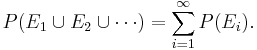
This is the assumption of σ-additivity:
- Any countable sequence of pairwise disjoint (synonymous with mutually exclusive) events
 satisfies
Some authors consider merely finitely additive probability spaces, in which case one just needs an algebra of sets, rather than a σ-algebra.
Consequences
From the Kolmogorov axioms, one can deduce other useful rules for calculating probabilities.
Monotonicity

The probability of the empty set

The numeric bound
It immediately follows from the monotonicity property that

Proofs
The proofs of these properties are both interesting and insightful. They illustrate the power of the third axiom, and its interaction with the remaining two axioms. When studying axiomatic probability theory, many deep consequences follow from merely these three axioms.
In order to verify the monotonicity property, we set  and
and  , where
  for
for  . It is easy to see that the sets
  are pairwise disjoint and
  . Hence, we obtain from the third axiom that
Since the left-hand side of this equation is a series of non-negative numbers, and that it converges to  which is finite, we obtain both
  and
and  . The second part of the statement is seen by contradiction: if
  then the left hand side is not less than
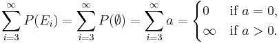
If  then we obtain a contradiction, because the sum does not exceed which is finite. Thus,
  . We have shown as a byproduct of the proof of monotonicity that .
More consequences
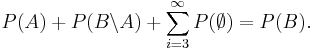
Another important property is:

This is called the addition law of probability, or the sum rule. That is, the probability that A or B will happen is the sum of the probabilities that A will happen and that B will happen, minus the probability that both A and B will happen. This can be extended to the inclusion-exclusion principle.
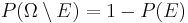
That is, the probability that any event will not happen is 1 minus the probability that it will.
See also
- Cox's theorem
- Law of total probability
- Measure Theory
- Borel Algebra
- σ-Algebra
- Probability theory
- Set theory
- Conditional probability
Further reading
- Von Plato, Jan, 2005, "Grundbegriffe der Wahrscheinlichkeitsrechnung" in Grattan-Guinness, I., ed., Landmark Writings in Western Mathematics. Elsevier: 960-69. (in English)
- Glenn Shafer; Vladimir Vovk, The origins and legacy of Kolmogorov’s Grundbegriffe, http://www.probabilityandfinance.com/articles/04.pdf
External links
- The Legacy of Andrei Nikolaevich Kolmogorov Curriculum Vitae and Biography. Kolmogorov School. Ph.D. students and descendants of A.N. Kolmogorov. A.N. Kolmogorov works, books, papers, articles. Photographs and Portraits of A.N. Kolmogorov.